Introduction
Let's motivate all of this with an example. Imagine you own a bike rental company. As an owner, a primary concern of yours would be about how much supply (i.e. bikes) to keep on hand; too much supply and you have invested money that isn't yielding enough of a return, and with too little supply, you are missing out on some potential profits because you will have to turn customers away. Balancing this equation is a classic problem for many businesses.
As you go about investigating what a good answer to this question is, you will probably consider different factors that affect bike supply. You begin to gather data so that you make an informed decision for your company. A variable that is clearly related to the number of bike rentals is temperature. If it's warmer, more people rent and if it's colder, less people rent. And this variable isn't static -- it changes throughout the day! Moreover, if it's mid day and warm, you are likely to get more renters than say if it's 8 pm and the same temperature (i.e. we get a kind of quadratic effect). Intuitively, this means that the effect of the same temperature isn't the same throughout the day! Temperature data is also good for another reason -- it's generally cyclic for the region you're in; this makes it easier to make supply decisions say, a year in advance without their being too much volatility with respect to the data with which you're making that decision.
Okay, so we've set up a problem -- you want to know the effect of temperature throughout the day on bike rentals so you can make decisions about how many bikes to keep at hand. We're going to solve this problem using Functional Neural Networks (FNNs). The set up will be to build up to FNNs and provide examples in this (bike rental) context. Essentially, we'll reason our way through this problem as each aspect of the method is introduced.
Functional Neural Networks
Neural Networks
Let's dive into neural networks first -- what are they? The simple answer is that they are big functions. You put something in and you get something out. In our case, we are going to put in daily temperature data and get out a prediction for the number of bike rentals on that given day. To really understand this, we have to expose ourselves to a bit of jargon.
Neural networks are made up objects called "layers" and "neurons" and these things connect to each other in a specific way. Each layer has some number of neurons. For example, the first layer might have 10 neurons, the second might have 15, and so on. The number of layers and the number of neurons in each layer is a "hyperparameter" which is a fancy word for saying that the user picks how many of each. Let's take a look at a single neuron.
$\begin{align} v^{(1)}_{3} = g\left(\boldsymbol{w}^{(1)}_{3}\boldsymbol{x} + b^{(1)}_{3}\right). \end{align}$
Let's really examine what's going on in this equation. The first part, $v_{3}^{(1)}$ will be the output. Notice that there are two numbers attached to $v$. The superscript (1) is a reference to the layer number and the subscript 3, is a reference to the neuron: this is going to be the output of the 3rd neuron in the first layer! An output here means just a single number. If we have say 15 neurons (subscript) for this first layer (superscript), then we will have 15 numbers come out of this first layer: $\boldsymbol{v^{(1)}} = \{v^{(1)}_{1}, v^{(1)}_{1}, ..., v^{(1)}_{15}\}$ where the bolded $v$ means that we are talking about a group of numbers i.e. a vector.
Next, let's talk about what $\boldsymbol{x}$ is here. Immediately, we can observe that it's bolded implying that this is going to be a vector and it is: it's our input. This is what we are putting into our network so that we can use this information to get an output. In our example, the input was daily temperature data. How we input this depends on what format the data is -- this is key. Perhaps the easiest way to think about this is hourly readings; so, for each hour, we have a reading of the temperature, and this information is available for all 24 hours in the day. This would mean that the vector $\boldsymbol{x}$ is 24 numbers. As a point of clarity, remember that our ultimate output is just going to be our prediction for bike rentals for a given day which means that the paired input (with each of these outputs) will be the 24 temperature readings for that given day.
Okay, so we know what $v$ and $\boldsymbol{x}$ are. Let's now understand $\boldsymbol{w}$ and $b$. First, the superscripts/subscripts (again) just correspond to a particular layer and a particular neuron. The vector $\boldsymbol{w}$ is what's known as the weights and these operate exactly as they are named. Remember that we are interested in how temperature affects total bike rentals but, we know that temperature is different at each hour -- therefore, the effect will also be different at each hour. What these weights tell you is what that effect is. Since we have 24 values of temperature, we're going to have 24 values of weights each of which will correspond to one of the hours. Imagine that $\boldsymbol{w}$ is the same value across all its 24 values; this would mean that it doesn't matter what time of the day it is, the only thing affecting the total bike rentals is the raw temperature data itself. It would imply that if you had say a reading of 18 degrees at noon and 18 degrees at midnight, that bike rentals would be affected in the same way -- this is of course, silly! So, what the network does is find out the different effect at each hour through a process called backpropogation (which I will omit details of). The value of $b$ AKA the bias is determined in a similar way -- this is an intercept term, it just shifts the value of $\boldsymbol{w\cdot x}$ up or down.
Finally, the last piece of this puzzle is $g()$. This is referred to as the "non-linear" part of the neural network. This is just some function that transforms the value inside and ultimately, is a part of why neural networks are considered "universal approximators". We can write all of this more compactly for an entire layer as follows:
$\begin{align} \boldsymbol{v}^{(1)} = g\left(\boldsymbol{W}^{(1)}\boldsymbol{x} + \boldsymbol{b}^{(1)}\right). \end{align}$
All we have done here is remove the neuron subscripts and the reason is because this equation represents all the neurons (for a given layer)! Think about when we looked at $\boldsymbol{v^{(1)}}$ -- the equation above gives us this vector but the equation I initially introduced only gave us the 3$^{rd}$ number in this vector. Also, before, when we looked at $\boldsymbol{w}$, it had 24 numbers (in our example); now, $\boldsymbol{w}$ has becomes $\boldsymbol{W}$ i.e. it is now a matrix. It now has 24 numbers in EACH row and has rows equal to the number of neurons. So, if we had 10 neurons, then the dimensionality of $\boldsymbol{W}$ is $10$ x $24$. Moving on, this process is repeated i.e. the output from this layer ($\boldsymbol{v^{(1)}}$) becomes the input to the next layer!
$\begin{align} \boldsymbol{v}^{(2)} = g\left(\boldsymbol{W}^{(2)}\boldsymbol{v}^{(1)} + \boldsymbol{b}^{(2)}\right) \end{align}$
This is done until the layer in which we get our predictions i.e. the final layer. If the goal is scalar prediction, there will only be 1 neuron (because you're only predicting one number). The backpropogation process alluded to earlier is how the network learns. By "learning", I mean that the network finds a better set of $\boldsymbol{W}$'s and $\boldsymbol{b}$'s so that the final output is closer to the what the observed value (e.g. bike rentals) should be.
Functional Data
In all of this, we made a key assumption -- we assumed that $\boldsymbol{x}$ is finite i.e. we know the vector $\vec{x}$ is going to be of some size $p < \infty$. In our example, we had a reading for each hour of the day so the size of the vector is 24. If we had readings at every half hour, then the size of our vector would be 48. Every 15 minutes and it becomes 96. What if we a reading at every possible time of the day? This is an infinite number of numbers. We know that practically, we can't work with $\infty$ in this way: how do you update an infinite number of weights? You don't.
All of this is a reference to functional data. I've written an introduction to this topic, but the gist of it is that, for example, instead of looking at each of the 24 hours as separate observations, we're only going to consider a single observation -- a functional observation, $x(s)$. This is basically a smooth curve built using the underlying data. The main assumption here is that this data we observe arises from some phenomenon and we would rather use a function that approximates that phenomenon than use the discrete observations. There are a number of advantages to this approach such as access to derivatives and the ability to measure our variable (temperature) at any point along the domain. For example, we wouldn't be limited to the temperature at 3 pm -- we would have information about what the temperature was at 3:31 pm or any time before or after!
Before moving on, let's introduce some notation. Let $x(s)$ be the functional observation -- this is our functional representation of the raw data points:
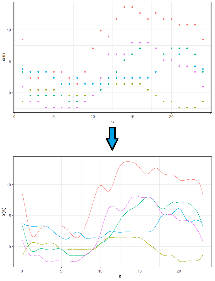
So, on the top plot, we have the raw temperature data whereas at the bottom is the functional observations (made using Fourier basis functions). Instead of passing on all the single points in the top plot, we will instead pass in the corresponding curve into the functional neural network.
FNNs
We now have the required background so let's get right into it. Our input is a curve ($x(s)$) rather than a vector ($\boldsymbol{x}$) so our weight is going to be a curve as well, say $\beta(s)$. However, updating a function is hard, so we do the following:
$\begin{align*} \label{eq2} v_{n}^{(1)} &= g\left(\int_{\mathcal S} \beta_{n}(s)x(s)ds + b_{n}^{(1)}\right)\\ &= g\left(\int_{\mathcal S} \sum_{m=1}^{M} c_{nm}\phi_{nm}(s)x(s)ds + b_{n}^{(1)}\right)\\ &= g\left(\sum_{m=1}^{M} c_{nm}\int_{\mathcal S}\phi_{nm}(s)x(s)ds + b_{n}^{(1)}\right), \end{align*}$
We're talking about the $n^{th}$ neuron of the first layer here. If you remember before, we were taking a linear combination of our input -- this is a sum. Now, we have an infinite amount of numbers so to take a sum here means to take an integral hence why the integrand shows up. The domain of the integral, $\mathcal{S}$ is dependent on the context. In our case, this will be from 1 to 24 as we are talking about the temperature throughout the day. In the second step, we rewrite the functional coefficient, $\beta(s)$ as a linear combination of M basis functions -- the same as we would do with the functional observations. So, to be clear, there are two linear combinations here -- one for $\beta(s)$ and one for $x(s)$. Then, in the third step, we swap the integral and the sum (trust me, we can do this).
Well, this is great. All we have to do now is update the coefficients ($\boldsymbol{c}$) of the basis expansion for $\beta(s)$; these are just scalar values so we can use all of the usual optimizatio schemes.
We can now generalize. What if we had other additional covariates. So, in our example, what if for each day, along with the temperature curves, we also had precipitation curves or, what if we wanted to pass in the temperature along with its derivative (a separate curve) -- implementing information like this simultaneously is what is meant by generalization in this context. This also extends to scalar covariates; we may know information about the day that isn't a curve e.g. we could have a scalar covariate $z_{1}$ that indicates what season of the year it is -- we may also want to use this information in our model (because it would help explain seasonal variation in the response). In other words, our input is:
$\begin{align*} \text{input} = \{x_{1}(s), x_{2}(s), ..., x_{K}(s), z_{1}, z_{2}, ..., z_{J}\}. \end{align*}$
The architecture of which looks like:
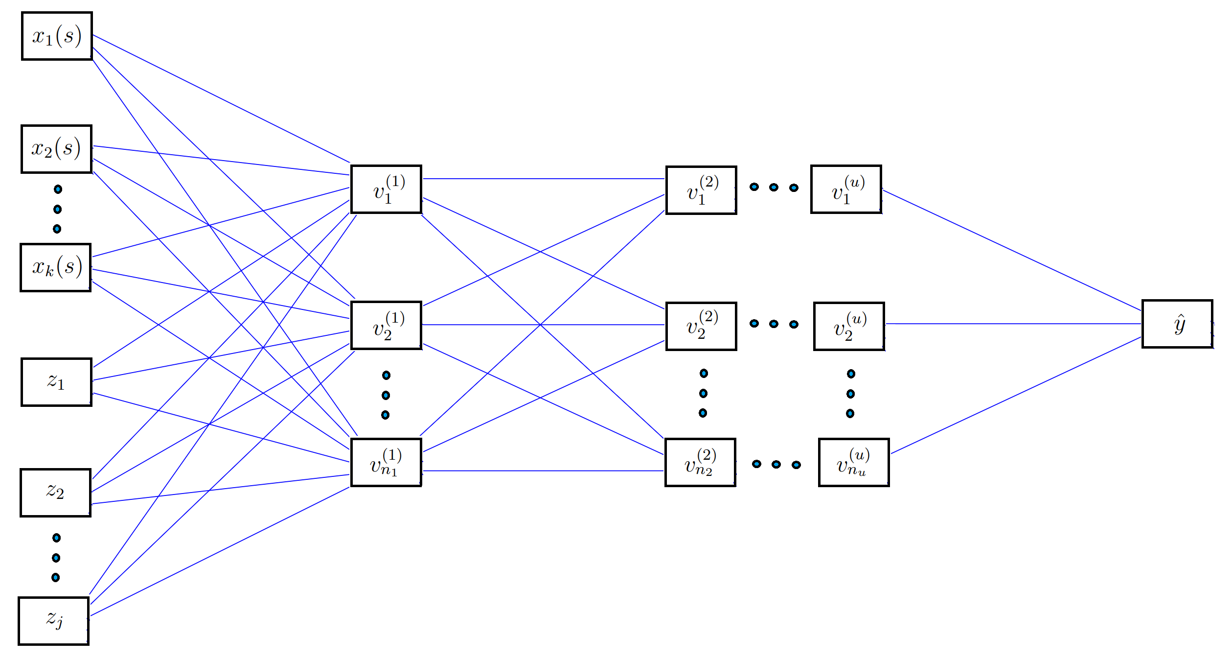
And, the form of each neuron now becomes:
$\begin{align*} v_n^{(1)} &= g\left(\sum_{k = 1}^{K}\int_{\mathcal S} \sum_{m = 1}^{M_k}c_{kmn}\phi_{kmn}(s)x_{k}(s)ds + \sum_{j = 1}^{J}w^{(1)}_{jn}z_{j} + b^{(1)}_n\right)\\ &= g\left(\sum_{k = 1}^{K}\sum_{m = 1}^{M_k}c_{kmn}\int_{\mathcal S} \phi_{kmn}(s)x_{k}(s)ds + \sum_{j = 1}^{J}w^{(1)}_{jn}z_{j} + b^{(1)}_n\right). \end{align*}$
All we have done here is added an additional term for the scalar covariates and, for the functional covariates, there is now an additional sum where each term corresponds to one of the $K$ functional covariates. For example, if we were using temperature, its derivative, and precipitation, then $K$ would be 3. This form of the neurons has justification in that we have shown it is a universal approximator. Observe that if you were to remove the first term within the neuron, you would recover back the usual neural network.
There are two final points before we get back to the bike rental problem. Remember that the weight function $\beta(s)$ on the functional observation is itself a curve. This means that we can observe how it changes as the network learns! It's much easier to look at a curve in the beginning (some random intialized curve) and then see how it changes over learning iterations. We dub these as functional neural coefficients. This is, at the risk of sounding too grand, a step inside the black box of neural networks. In the usual case, we would just have numbers ($\boldsymbol{W}$ and $\boldsymbol{b}$) and we could theoretically make some effort in trying to figure out why they change in the way that they do but, when you have thousands of these numbers, it becomes a near impossible task. We'll see this interpretive advantage of FNNs in action in the next section.
The second point concerns the parameter count. In the case of the usual neural network, if we passed in the discrete points for the day, then there would be 24 weights for each neuron in the first layer. In the functional case, the weights are dependent on the choice of $M$ which is the number of basis functions defining the functional neural coefficient, $\beta(s)$. There is no need for $M$ to be big and often, for the sake of smoothing and for the purpose of not overfitting, $M$ is chosen to be rather small (in our case, this choice will be a hyperparameter). Say we let $M = 5$, then we have have a reduction of 24 - 5 = 19 weights within each neuron of the first layer! In essence, we'll see that we will get better predictions using fewer parameters -- kind of an incredible thing!
Analyzing the Bike Rental Problem
That was a lot but we're finally ready to get back to the problem at hand. Our goal is to predict the number of bike rentals using temperature curves. Let's first use the usual neural network. We can visualize the weights by seeing how they move as we train the network. We'll see that the error goes down but the network weights themselves aren't all that interpretable.
What's happening here is that the model is improving as indicated by the decreasing error plot on the right hand side. On the left hand side is the weights associated with just one of the neurons of the network and what their values are at a particular training iteration. The relationship between the hourly temperature and bike rentals isn't as intuitively clear with these set of weights. We observe that the underlying autocorrelation structure isn't preserved either i.e. there should be some smoothness between adjacent hours but, in the final estimated weights, there seem to be jumps hour to hour. For example, you might be hard pressed to explain the low weight at 3 pm because it's sandwiched by high weights at 2 pm and 4 pm. Also, the general shape across the day is harder to explain than what we will get with the analysis we're about to do next!
Let's not analyze this problem through FNNs. We are going to pass in curves and plot the functional neural coefficient:
We don't have individual weights now -- we have just a curve across the continuum that is changing as the network trains. The associated error with this model is on the right hand side (it's hard to tell, but it's actually lower than regular neural network model). Let's take a closer look at what the functional neural network is outputting; we can observe that the network begins at some random initialization and, as the network learns, we get a curve that seems to have the most minimal effect from midnight to about 6/7 am. The effect also begins to drop off rapidly in the evening. This makes sense because it's telling us that the temperature at those times is not all that impactful on bike rentals -- the store is closed those times so there shouldn't be much of an effect!
We can also observe a quadratic relationship as a function of the time. As we get closer to the afternoon, the effect increases rapidly -- this is telling us that a sunny morning likely decides whether someone will go rent a bike; perhaps they make this decision in the morning and then actually arrive at the store around noon -- this is reasoning that is inline with what we would expect of human behaviour (maybe it's colder in the morning, or the weather just happens to be the best, on average, in the afternoon). Finally, observe when the error begins to taper off (in how much it decreases) -- it's associated with when the functional neural coefficient is adjusting the tails i.e. when we see the least effect on rentals. On the other hand, the model error decreases the most when the network adjusts the part of the curve associated with the actual open hours of the store. None of this interpretation is available from the regular neural network! Here is a model that has less parameters, has a lower error rate, and is more immediately interpretable. The final results from the paper showed that just using these temperature curves explained about 65% of the variation in daily rentals (as measured by $R^2$) and had the lowest cross-validated error rate -- this bested several other models!
Oh, and this plot?
Well, this is just the functional neural coefficients associated with a model using the temperature curves along with the first two derivatives as the functional covariates (i.e. $K = 3$). You can try and make sense of them yourself!
Conclusions
In our paper, we have many more results and details about this example and others. The goal here was to provide an intuitive explanation of what's going on with these networks and why they can be useful. This is a machine learning tool for longitudinal data -- a field that seems to lack methods like this. We are working on a paper that extends this to curve responses as well! To temper some of the claims here, I will say that this (as you might have guessed) doesn't work everytime -- the estimated functional neural coefficient may, at times, not have any clear interpretation; this is just a consequence of the optimization procedure. Moreover, there will definitely be cases where other methods will do a better job of explaining variation and/or have lower error rates (which is just the nature of modelling in this way). Regardless, we present here a method that comes with a number of benefits and is, at the very least, a new toy in any modellers' arsenal. Oh, and the best part is that we're developing a package i.e. a chance for anyone could to use these methods with their own data sets; look for that sometime this summer!